MOLE 2.0

Tunnel search with MOLE 2.0 and MOLEonline 2.0

In short, a tunnel is a path between a point inside the macromolecular structure and its boundary. A tunnel is formed by its centerline and profile that specifies tunnel radius in each of centerline points.

In essence, to find a tunnel the previous version of MOLE required the user to specify a starting point and from this point, the graph formed by the dual of the Delaunay triangulation (the Voronoi diagram, see bellow) got traversed in a depth first manner (paths with the lower cost were visited first). Each time a boundary vertex was reached, a tunnel got reported.

There are numerous problems with this approach. For example, when the first tunnel got reported, the next one was very similar to the first one (and therefore provided no useful additional information) because the path "branched" near the end point of the first tunnel. Another issue was caused by small "ridges" that were formed by vertices near the boundary of the diagram. As a result, a large part of the tunnel was often "going along" the surface of the protein and therefore they didn't provide a very relevant information about the structure of the tunnel. It was also very difficult to identify interesting starting points of the tunnels, unless prior knowledge.

The current version of the new MOLE 2.0 algorithm addresses these problems issues by preprocessing the Voronoi diagram, splitting it into several smaller parts (called cavity diagrams) and identifying suitable start and end points. Finally, Dijkstra's algorithm is used to find the tunnels. This algorithm is used also in MOLEonline 2.0 web application.

MOLE 2.0 algorithm overview

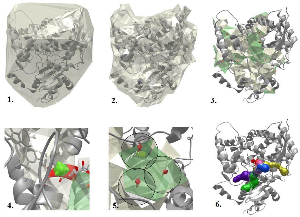
The tunnel computation in MOLE 2.0 is performed in several steps:

• 1. Calculate the Delaunay triangulation/Voronoi diagram of the atomic centers.
• 2. Approximate the molecular surface by removing tetrahedrons that are too big. A tetrahedron is too big if a sphere with the Probe Radius can fit through it. Therefore, the smaller the Probe Radius is, the more tetrahedrons get removed.
• 3. Find cavities - remove tetrahedrons that are too small and identify connected components from the remaining tetrahedrons. A tetrahedron is too small if a sphere with the Interior Threshold radius cannot fit through it.
• 4. Identify the start point as the closest tetrahedron in a cavity that is within the Origin Radius distance from the selected residues. If there is no such tetrahedron, no tunnel can be found in the given cavity. This is done separately for each cavity.
• 5. Identify end points by covering boundary components of the cavities by a set of spheres with the Surface Cover Radius r. The distance between all pairs of end points is in the interval <r,2r>.
• 6. Compute the tunnels as shortest paths between all pairs of start and end points (that are in the same cavity). If two tunnels are too similar, the longer one is not reported.

1. Macromolecular Voronoi diagram representation

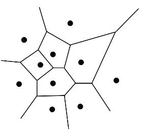
The Voronoi diagram divides a metric space according to the distances between discrete sets of specified objects. In MOLE 2.0 case objects are the centres of the atom with van der Waals spheres. vdW radii of the spheres are taken from AMBER force field. The edges of the diagram represent equidistant positions between pairs of the closest atoms. The Voronoi diagram can be computed as a dual of the Delaunay triangulation of vdW sphere centers. Therefore, the vertices of the diagram correspond to the tetrahedrons of the triangulation and are located at the tetrahedrons' circumcenters. Similarly, the edges of the diagram represent the adjacency of the tetrahedrons.

2. Preprocessing the diagram

The preprocessing works in several steps:

• The boundary of the Voronoi diagram corresponds to the convex hull of the protein. This is not desirable because then the tunnel exits might end up being too far from the actual protein surface (similarly the shallow ridge issue of the previous algorithm). To remedy this, the user is required to specify the probe radius parameter which is used to approximate the molecular surface. Given this parameter, layers of vertices are removed repeatedly starting from the boundary layer if the probe would pass through corresponding tetrahedron.This process is repeated as long as there is no longer any vertex to remove.
• The second step is the removal of vertices of the Voronoi diagram (i.e. tetrahedrons) that cannot be part of any tunnel. This is governed by a parameter called the interior threshold. This parameter serves as an approximate lower bound on the tunnel radius. A vertex is removed if a sphere with the interior threshold radius cannot pass through any of the tetrahedron's sides.
• After the boundary and interior vertices are removed, the cavity diagrams are computed as the connected components of the Voronoi diagram. In essence, these cavity diagrams represent the empty space inside the macromolecule.
• The last preprocessing step is to remove the shallow vertices. These are the vertices that form the above mentioned ridges along the surface of the molecule. All vertices with the distance (defined simply as a the number of the vertices on the path) from the surface less than a given internal threshold 5 are removed if all their neighbors have the same or lower depth.

3. Detection of Start points and End points

Once the diagram is split into several smaller cavity diagrams, these are analyzed for suitable tunnel start points and end points between vertices of the cavity. The general idea here is that the start point is the "deepest" vertex in the cavity and the end point is the "largest" boundary vertex (i.e. corresponding to the largest tetrahedron).

Start Points

There are two ways to specify a start point for a tunnel - user specified list of residues, XYZ coordinates or (MOLE 2.0 only) automatic computation:

• User defined:

The user specifies a list of residues or a 3D point. Next, the centroid calculated from all the corresponding atomic centers is computed. Finally, for each cavity within a specified origin radius the closest vertex is selected as a start point.

• Calculated: (MOLE 2.0 only)

The topology of the cavity is used to calculate the start point. The calculated starting point is the "deepest" vertex of a cavity. The depth of a vertex is defined as the length of the path from this vertex to the closest boundary vertex.

End Points

Similarly to the start points, endpoints are either user defined (MOLE 2.0 desktop version only) or calculated:

• User defined:

These end points can be specified by clicking on the surface of the molecule in MOLE 2.0 desktop aplication.

• Calculated:

For each cavity diagram a subgraph B is induced by the boundary vertices. Then, the connected components of B are computed. Finally, each component is covered with spheres with the surface cover radius and the tetrahedrons corresponding to the centers of these spheres are marked as tunnel exits.

4. Tunnel computation

Finally, when the set of start and end points is identified for each cavity, the Dijkstra's Shortest Path algorithm is used to find the tunnels between all pairs of start and end points points (or the molecular surface if the algorithm reaches it before it finds the tunnel exit). The edge weight function used in the algorithm takes into account the distance to the surface of the closest vdW sphere and the edge length.

Then the tunnel centerline is represented as a 3D natural spline representation defined by the Voronoi diagram vertices that form the path found by the Dijkstra's algorithm.

Because of the density of the computed exits, the algorithm might find duplicate tunnels. Therefore, in the last post-processing step, these duplicate tunnels are removed.

Assignment of physico-chemical properties

When tunnel is shown, a set of unique residues lining it is shown, while those surrounding the tunnel with side chain are noted. According to side chain, a list of properties is calculated (for lining aminoacid side chains only):

• Charge is calculated as a sum of charged residues (Arg, Lys, His = +1; Asp, Glu = -1)
• Hydropathy of the tunnel is calculated as an average of hydropathy index assigned to residues according to the method of Kyte and Doolitle. (Kyte, J. and Doolittle, R.F., A simple method for displaying the hydropathic character of a protein, J. Mol. Biol. 157, 105-132 (1982)). Hydropathy index is connected with hydrophilicity/hydrophobicity of amino acids (most hydrophilic Arg = -4.5, most hydrophobic Ile = 4.5).
• Hydrophobicity is calculated as an average of normalized hydrophobicity scales by Cid et al. (Cid, H. et al. Hydrophobicity and structural classes in proteins, J Protein Engineering 5, 373-375 (1992)). Most hydrophilic residue according to hydrophobicity value is Glu (-1.140) and the most hydrophobic is Ile (1.810).
• Polarity is calculated as an average of amino acid polarities assigned according to the method of Zimmerman et al. (Zimmerman, J.M. et al. The characterization of amino acid sequences in proteins by statistical methods, J. Theor. Biol. 21, 170-201 (1968)). Polarity ranges from completely nonpolar aminoacids (Ala, Gly = 0.00) through polar residues (e.g. Ser = 1.67) towards charged residues (Glu = 49.90, Arg = 52.00).
• Mutability is calculated as an average of relative mutability index (Jones, D.T., Taylor, W.T. and Thornton, J.M. The rapid generation of mutation data matrices from protein sequences, Comput Appl Biosci (1992) 8 (3): 275-282.). Relative mutability is based on empirical substitution matrices between similar protein sequences. It is high wherever aminoacid can be easily substituted for another e.g. in case of small polar amino acids (Ser = 117, Thr = 107, Asn = 104) or in case of small aliphatic amino acids (Ala = 100, Val = 98, Ile = 103). On the other hand it is low when amino acid plays important structural role such as in case of aromatic amino acids (Trp = 25, Phe = 51, Tyr = 50) or in case of special amino acids (Cys = 44, Pro = 58, Gly = 50). Specific example of amino acid with low relative mutability is the most abundant amino acid (Leu = 54) which has the highest probability to mutate back to itself.

Note on advanced options

Advanced settings offers possibility to adjust parameters determining tunnel searching algorithm. All parameters are set in Angstroms (0.1 nm):

• Probe radius - Radius used for construction of surface of biomacromolecule.
• Interior threshold - Approximate smallest tunnel radius to use.
• Surface Cover Radius - Determines the density of tunnel exits on the molecular surface.
• Origin radius - Localization of starting point within this radius.
• Starting point [X,Y,Z] - Precise localization of starting point instead of list of residues.

Final Note on the complexity of the algorithm

The worst case complexity of the algorithm is O(M log M) where M is the number of vertices of the Voronoi diagram. In the worst case, M = N², where N is the number of atoms. However, in most practical cases M is almost equal to N. Additionally, the complexity of calculating the Voronoi diagram is O(N log N). The complexity of all steps of the pre-processing phase is at most O(M log M). Finding the paths using the Dijkstra's algorithm is O(K M logM) where K is number of tunnels.

Together, the complexity of the MOLE 2.0 tunnel search algorithm is O(K N² log N), where K is the number of detected tunnels and N is the number of atoms in the molecule.